Kelly criterion and investing
Kelly criterion is a mathematical formula used to specify how much a player faced with a series of bets should risk on every single one of them to maximize long-term growth.

Kelly criterion is a mathematical formula used to specify how much a player faced with a series of bets should risk on every single one of them to maximize long-term growth.
It was discovered and featured by a researcher from Bell Labs, J. L. Kelly, Jr in 1956. Surely such formula must be useful in most gambling scenarios, but under some additional assumptions, it can also be adapted to the investing setup.
First, I’ll take a look at what Kelly criterion is why do we need it at all. Next, I’ll simulate some hypothetical scenarios and measure how does the formula perform. In the last part, I’ll validate it with some real-world stock-market data.
A gambling example
When one goes to a Wikipedia entry[1] to read about a Kelly criterion, in one of the first paragraphs a fascinating story can be found:
In one study, each participant was given $25 and asked to bet on a coin that would land heads 60% of the time. The prizes were capped at $250. "Remarkably, 28% of the participants went bust, and the average payout was just $91. Only 21% of the participants reached the maximum. 18 of the 61 participants bet everything on one toss, while two-thirds gambled on tails at some stage in the experiment. Neither approach is in the least bit optimal."
When we follow the links a bit, we can find the reference to the original paper that describes the experiment[2]. It reveals, that these weren't ordinary people who were offered to participate:
The sample was largely comprised of college age students in economics and finance and young professionals at finance firms. We had 14 analyst and associate level employees at two leading asset management firms.
These were people learning to become or already being professional money managers. 28% of them went bust, while 21% reached the maximum amount of $250.
Let's see if, with some help of mathematics, we can try to beat them.
A bit of mathematics
Like any other mathematical formula, Kelly criterion needs some assumptions to be satisfied. In the most simple case, we need:
- A series of identical bets – long enough that long-term statistical properties show from the short term noise.
- Two outcomes: either winning the payoff of \(W\) times the amount we've bet with probability \(p\) or losing the bet with probability \(1 - p\).
- Ability to scale the bet, so that we can bet any amount we have at our disposal (no limits how much/how little we can bet).
And that's it. Nothing more. The most important part here is that we must know the probability distribution beforehand. If we know it exactly, we can calculate the optimal bet size. Without knowing the odds exactly, the formula will be of no help.
In the study mentioned in the previous section, participants had 30 minutes to place as many bets as they wanted, but in our case, we'll limit that number to 300. To wrap the situation in some concrete numbers we have:
- The probability of winning is \(p = 60\%\), so the probability of losing equals \(q = 1 - p = 40\%\).
- In case we win, we receive the amount of bet so \(W = 1\), if we lose, we must pay the same amount.
- We toss the coin \(N = 300\) times.
We're ready now to present the formula that we've talked about so much. It doesn't look very impressive, but let's not judge the book by it's cover – we'll judge it by the results.
\[ f_* = \frac{\textrm{expected bet payoff}}{\textrm{bet payoff in we win}} \]Expected bet payoff is how much on average we would get if we made this bet a large number of times with the same capital.
We can already have a few conclusions from this formula:
- \(f_*\) is always smaller than 1: we can never bet more money than we have – that sounds reasonable
- \(f_*\) is positive (meaning we bet any money) only when an expected payoff is positive. It's not possible to win (long-term) betting on a game with negative expected payoff. That's why one cannot get rich betting in a casino, but the stock market has created a few fortunes.
Substituting symbols in the formula for actual data, we have:
\[ \begin{align*} f_* &= \frac{p \cdot W + q \cdot (-1)}{W} = \frac{p \cdot W - (1 - p)}{W} \\ &= \frac{p (W + 1) - 1}{W} = \frac{0.6 (1 + 1) - 1}{1}\\ &= 1.2 - 1 = 0.2 = 20\% \end{align*} \]And that's the whole story – with each flip we should bet \(20\%\) of our money to maximize our return. If we win – we bet a bit more in the next round (because we have more capital), if we lose – a bit less.
Let's simulate some coin flips and see how Kelly strategy would perform on this problem. I've made ten random runs of 300 bets per person, and plotted the amount of money each person had after each bet:
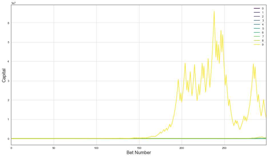
Wow, it turns out one lucky person has around $10 million in winnings, which made other series look so tiny that they’re basically the same line on the graph. It is actually quite surprising to see how much money one can win with just 300 slightly biased coin tosses and $25. To investigate in more detail how each player was doing throughout the game, let’s look at this graph on the logarithmic scale - where one step from a tick mark to the next one on the y-axis means multiplication by 10.
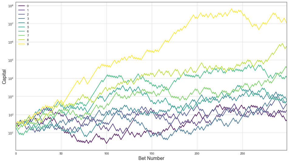
That’s a bit better overview of what’s actually going on. We can definitely see that the game is quite risky: some people have won a lot while the more unlucky ones have gotten much less (multiple orders of magnitude). Still, everyone has finished on top of what they’ve started the game with ($25). Let’s look at the table of winnings:
| Final capital | |
|---|---|
| 0 | 53.97 |
| 1 | 182.16 |
| 2 | 409.86 |
| 3 | 614.79 |
| 4 | 614.79 |
| 5 | 614.79 |
| 6 | 10504.19 |
| 7 | 35451.65 |
| 8 | 605724.76 |
| 9 | 10349375.40 |
But that’s just ten random examples – that’s not enough to make really firm conclusions. They could have just been lucky(unlucky?). I’ll simulate now a larger sample of 100’000 players and present you some statistics of that. Then, we can contract how we did we do compared to the group from the study.
This is the histogram of winnings of 100’000 random participants betting on the same 60/40 coin using Kelly methodology:
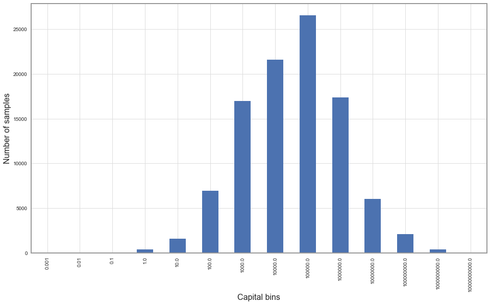
On the x-axis we can see the histogram bins – they’re also created with logarithmic spacing. E.g. a bin marked 100.0 above counts people who finished the game with capital between 10.0 and 100.0. Let’s extract some of the most interesting statistics and put them in the table:
| Count | Percentage | |
|---|---|---|
| Capital < 1.00 | 427 | 0.4% |
| Capital < 25.00 | 4436 | 4.4% |
| Capital > 250.00 | 86758 | 86.8% |
| Capital > 10'000.00 | 52493 | 52.5% |
| Capital > 100'000.00 | 25940 | 25.9% |
Only 0.4% of our large sample ended broke (capital less than $1) – Seems like we're outperforming the group from the experiment[2] quite heavily. Only 4% finished with less capital than when they've started playing. 87% of the sample had more than the prize cap set by the organizers - $250! More than half had over 10 thousand and more than a quarter over 100 thousand. That's quite a lot of winnings from 300 coin tosses.
The luckiest participant would leave with $4.5 billion, if there were no cap on the winnings – we can clearly see why did the organizers put it in! If they didn't, and participants would play with Kelly strategy, they would have to pay on average over $2 million per person. That would make it an overly expensive research.
It is useful to notice how strongly positively skewed the outcomes are: a small portion of participants gets huge payouts. The mean is two orders of magnitude larger than the median.
What if our probability estimations are wrong?
What if the experiment organizers lie to us? What if the coin was more biased or less biased than the organizers have told us? Mathematics proves that betting with Kelly methodology is in some sense optimal if we are right about the probability distribution and play long enough. The theorem itself, though, specifies very little about how does it perform when the probabilities differ from our views.
Let's perform some empirical tests of that.
I'll consider two different scenarios:
- Scenario I – coin lands heads (participant wins) 55% of the time
- Scenario II – coin lands heads 65% of the time
We could calculate easily Kelly ratios for each of above scenarios if we knew the real probabilities. They would be 10%, 30% respectively. I’ll compare that vs. investing 20% as in the 60⁄40 case.
I'll make a simulation of 10'000 cases of 300 coin throws and compare the betting performance of "misinformed" 20% bet vs. the Kelly optimum.
Scenario I
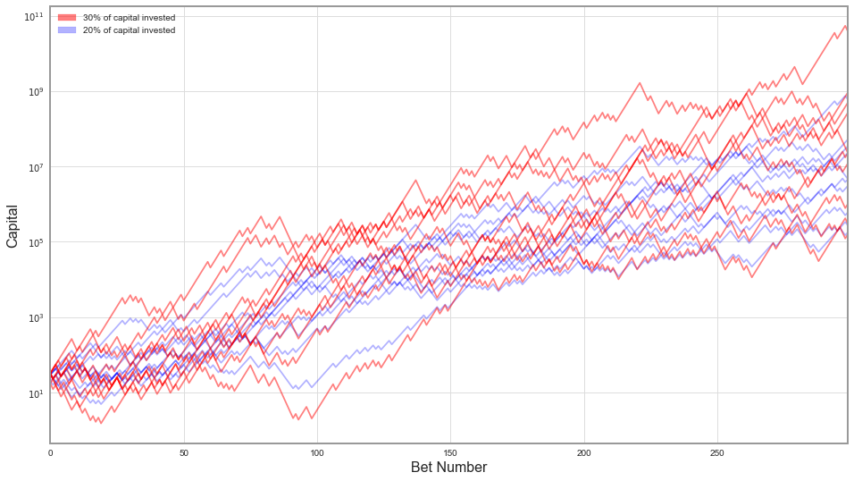
On below graph, I've made ten random coin flipping "runs" while investing 10% of capital in every bet (marked red) – optimal Kelly. On the other hand, marked blue are ones with 20% of capital invested in each bet.
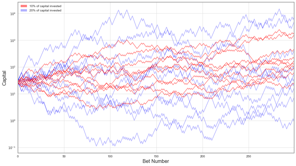
We can clearly see that having 20% of capital "invested" in each bet is riskier - with each bet we put more money at stake, but do we receive more reward for that? Blue lines are significantly more dispersed than the red ones, some of the blue runs finish with capital larger than the red ones, but also a prominent group ends with much smaller winnings.
Let's look at more detailed statistics from the larger sample:
| 10% | 20% | |
|---|---|---|
| Capital < $1 | 0.21% | 19.15% |
| Capital < $25 | 19.15% | 52.40% |
| Capital > $250 | 34.62% | 26.71% |
| Mean Winnings | 485.19 | 5652.01 |
| Median Winnings | 112.32 | 23.99 |
Out of the people were putting 10% of their capital on every bet, only 0.2% went broke throughout the game (that's one person out of five hundred). From ones that put 20%, it was 20% – one in five. That's quite a significant risk. More than half of the participants betting 20% ended the game with lower capital than they started.
An interesting paradox arises, when we take a look at the mean, or in other words, average winnings. Average in that context means that we take funds paid to all the participants and divide them by the number of participants. These are higher for a group who bet more – and in some sense that is expected. The game has a positive expected payoff, what entails that the more you bet the more you'll win on average. The important thing here is, that average tells us very little about the distribution, and in this case, the distribution is very strongly skewed. A few people who risk a lot will win colossal payoffs, but most will be worse off.
A median of payoff while betting 10% is five times larger than if we're betting too much.
Scenario II
Let's do the same analysis as above for when the coin has odds 65/35, and we bet either 20% or 30% of our capital.
The situation is significantly different here. The odds are so much better now, that basically everyone "wins", but people who bet more – win more. Again, that's expected. Let's see how much more.
| 20% | 30% | |
|---|---|---|
| Capital < $1 | 0.00% | 0.04% |
| Capital < $25 | 0.02% | 0.25% |
| Capital > $250 | 99.90% | 98.74% |
| Mean Winnings | 818 M | 1042 B |
| Median Winnings | 46 M | 225 M |
I've double checked these numbers, and I don't think I've made a mistake. Betting more makes you take on more risk - but very marginally in that case. Yet the difference in average winnings is huge. It's 800 million vs. 1000 billion (a trillion). That's three orders of magnitude more. Median is also almost five times larger.
What do we know so far
- We've applied the Kelly formula to the simple betting game.
- We have outperformed a group of finance students on betting with a biased coin.
- We have verified how betting with Kelly formula is doing when the outcome probabilities are not exactly the ones we believe in.
What turns out, is that if probabilities are worse than expected, we're taking considerably more risk by betting too much. That increases our chances of going broke or not earning any positive return. On the other hand, if the game is more favorable than we've assumed, we're giving away possible winnings.
It's time to move on to the stock market.
Stock market applications
Let's assume we already have a portfolio that we want to invest in - an S&P 500 Total Return Index. In the real world, S&P 500 is not directly investible, but there is multitude of tracker funds.
We also have a risk-free bond, for which I'll use a rolling 3-month US T-bill position.
I was able to get 29 years of data from Yahoo! finance for these instruments – for a period from 1988 until the end of 2016.
Previously, we asked ourselves how much of our capital should we put on a single coin-tossing bet. Now the question is different: how much of our money do we put on risky asset (S&P 500) vs. the risk-free one. We allow ourselves to borrow money at a risk-free rate as well, to leverage our equity position. Let's see what does the Kelly tell us to do.
There is a generalization of Kelly criterion for multiple risky assets, but it's not inherently different from constructing an optimal risky portfolio first and then deciding on the split of that vs. the risk-free asset. I'll focus on a single risky portfolio case then.
Kelly stock market formula
We have a risky asset with an annual rate of return \(\mu\), volatility \(\sigma\) and a risk-free bond yielding \(r\). How much do we invest in each? Kelly formula, again, turns out to be pretty simple:
\[ f_* = \frac{\textrm{mean excess return of risky asset}}{\textrm{volatility squared}} \]In the period from 1988 until 2016 we've experienced quite a few equity rallies and at least two sharp downturns. Overall, this timescale turned very beneficial for investors with S&P investing returning on average 8.08% above risk-free rate per year with annualized volatility of 17.67%.
Calculating the Kelly ratio we get:
\[ f_* = \frac{ 0.0808 }{ 0.1767 \cdot 0.1767 } = 2.59 \]A number greater than one means Kelly criterion is suggesting to invest more money than
we currently possess. Surplus needs to be borrowed at the risk-free rate. Let's consider a few different portfolios ordered from the least risky to the riskiest and analyze their performance in the timeframe discussed.
- Classical 60/40 portfolio: that is 60% of our capital will be invested in the stock market portfolio, and the rest stored safely in bonds. We'll treat the risk-free asset as a substitute for bonds in that case, for simplicity.
- Everything (100%) allocated to S&P 500 investment.
- Half Kelly - 130% of allocation to a risky portfolio. That means additional 30% of capital is borrowed.
- Full Kelly - 259% allocated to a risky portfolio.
- Double Kelly - 500% of capital allocated to a risky portfolio.
Let's look at the plot of cumulative returns of these investments:
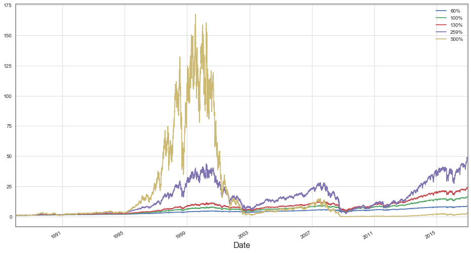
We can see that the hyperaggressive 500% investor went a few steps too far: at some point, he has achieved more than 150x return on his capital only to lose it all in a dot-com bubble.
Let's take a look at this chart in logarithmic scale:
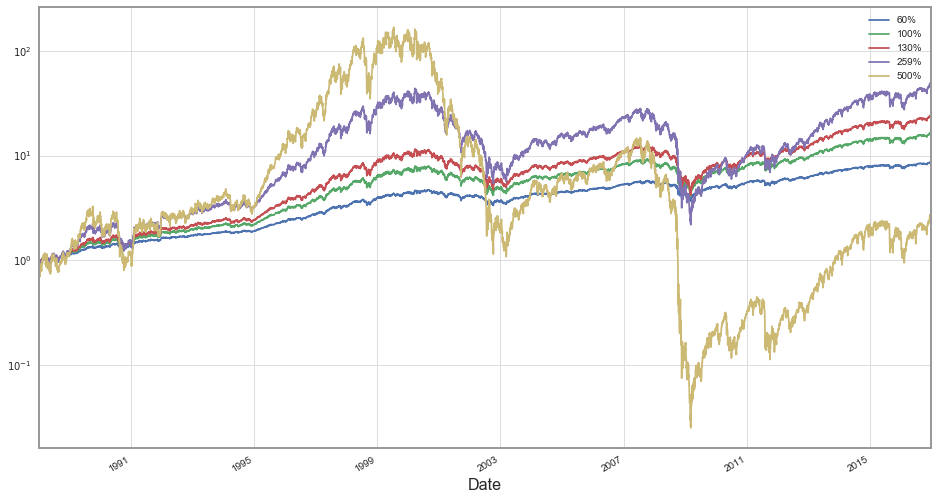
Clearly investing according to the kelly ratio wins both short term and long-term. Betting more aggressive than that turned out to be catastrophic while more conservative approach still paid out – just less. Below I'll put final return for each investor:
| Annual | Cumulative | |
|---|---|---|
| 60% | 7.7% | 8.6 |
| 100% | 10.1% | 16.2 |
| 130% | 11.5% | 23.7 |
| 259% | 14.2% | 47.3 |
| 500% | 3.3% | 2.5 |
Overall, the portfolio invested 500% in equities had return of 3% per yer – it's almost the same what would risk-free rate return. Interesting is the difference between Kelly and Half-Kelly, on an annual basis it's only 3% more but over 29 years that compounds to doubling the final capital.
Even investing very safely via a 60/40 portfolio turned out to be highly profitable – returning more than 7% each year.
Highly leveraged Kelly portfolio turned out to be the best choice in that case. But there is one caveat - we knew beforehand the mean return and volatility for the stock market so we knew the exact Kelly ratio we needed to invest to obtain optimal results. Just like I mentioned in the previous section, we don't always know the probability distribution of random games ahead. However, we never know, what the average return for the stock market will be in given future period. That makes investing significantly harder.
So yes – we've cheated to make Kelly portfolio win, and it won. Now let's make a comparison slightly fairer.
No looking back
I'll divide the data I have in two periods from 1988 until the end of 2001 and from 2002 to 2016. I'll use mean return and volatility from the first period to calculate the Kelly ratio for the second one.
Mean return in the first period was 9.1% percent above the risk-free rate with annualized volatility of 15.6%. The optimal fraction of capital invested according to Kelly is 3.75.
My new set of possible portfolios will be similar to the previous one, just rescaled to the new optimal ratio – one that a person looking to invest at the beginning of 2002 would determine, looking at the past fourteen years:
- Classical 60/40 portfolio
- Equities only (100%)
- Half Kelly - 187%
- Full Kelly - 375%
- Double Kelly - 750%
It turns out that our second period was much less favorable for investors than the first one.
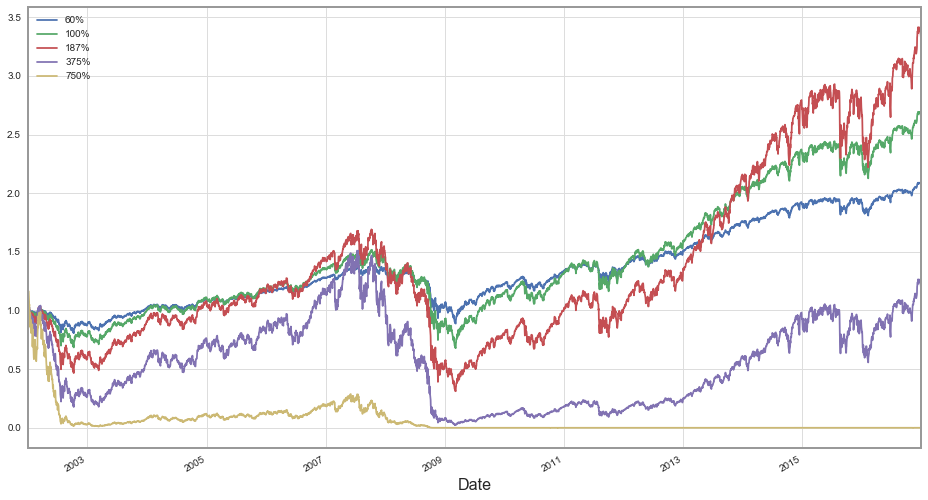
With a lower average return of 7.1% per year and higher volatility of 19.5% the times proved to be much more challenging. The most highly leveraged investor went broke almost instantly – through some aftermath of the dot-com bubble.
A portfolio constructed according to the Kelly methodology lasts slightly longer – to the financial crisis of 2008. The Half-Kelly methodology turns out to be the winner overall, with others lagging only slightly.
| Annual | Cumulative | |
|---|---|---|
| 60% | 5.0% | 2.1 |
| 100% | 6.7% | 2.7 |
| 187% | 8.3% | 3.3 |
| 375% | 1.2% | 1.2 |
| 750% | --- | 0.0 |
Conclusions & Closing remarks
I hope I've convinced you in the above article that Kelly criterion is the useful mathematical tool in analyzing random games and investments. If nothing more, it would allow us to beat a group of finance students in the coin-tossing game.
Still, when applied to investments, Kelly may suggest a highly risky position, especially when coming out of a calm period. That may be deceptive. We've analyzed several scenarios when we didn't know the exact probability distribution of our future payoffs. They've shown that if we're too optimistic in our modeling, by using Kelly formula we increase our risk of going broke significantly.
To sum up, if we are confident about the probability distribution of the game we're playing, betting according to the methodology presented here will outperform any other in the long-term. If we're not sure, betting half of the calculated ratio or even less may be advised.